
最近の技術発展はすさまじく、画像分類ごときは一瞬で作成できます。
初心者でもコードをコピペすれば実装できるので、やってみましょう。
Pythonの実行環境を持っていない人はGoogle Colaboratoryを使ってください。
>>Google Colaboratoryの使い方
データセット
そもそも機械学習に使える都合の良い画像を持っていない人もいますよね。
それでも大丈夫です。
すでに用意されているサンプルデータがあるので、これを使いましょう。
import torch
import torchvision
from torchvision.datasets import CIFAR10

train = CIFAR10(root = "data", download = True, transform = torchvision.transforms.ToTensor(), train = True)
test = CIFAR10(root = "data", download = True, transform = torchvision.transforms.ToTensor(), train = False)
CIFAR10という画像データをダウンロードできます。
“data”というフォルダができていれば成功です。
中身を見てみましょう。
import matplotlib.pyplot as plt
plt.figure()
plt.subplot(1, 2, 1)
plt.imshow(train[0][0].permute(1, 2, 0))
plt.title(train[1][1])
plt.subplot(1, 2, 2)
plt.imshow(test[0][0].permute(1, 2, 0))
plt.title(test[1][1])
plt.show()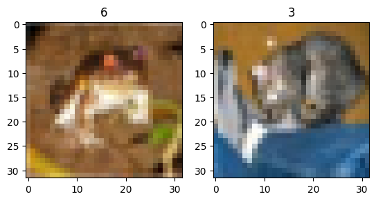
それぞれこのように32 x 32の画像が入っています。
写真の種類は数値ラベルで決まっています。
カエルが6で、3は猫らしいです。
plt.figure()
for i in range(9):
    plt.subplot(3, 3, i + 1)
    plt.imshow(train[i][0].permute(1, 2, 0))
    plt.title(train[i][1])
plt.tight_layout()
plt.show()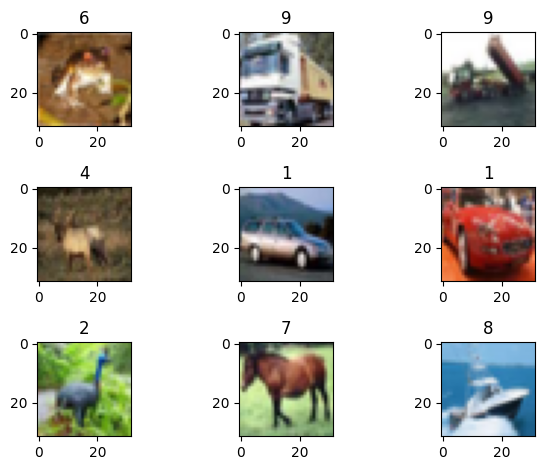
このように写真の種類別にラベルが振り分けられています。
CIFAR10は0~9までの10種類の画像があるデータセットです。
つまり、写真から番号を当てられればOKということです。
DataLoader
画像データは容量が重いので、バッチサイズを指定して小分けして処理します。
ようするに、一気に全部の画像を読み込むとパンクします。
train_loader = torch.utils.data.DataLoader(train, batch_size = 256, shuffle = True)
test_loader = torch.utils.data.DataLoader(test, batch_size = 256 * 2, shuffle = False)
batch_sizeが小出しする枚数です。今回は256にしました。
画像1枚ごとのデータ容量でbatch_sizeは調整します。
batch = next(iter(train_loader))
print(len(batch))
print(batch[0].shape, batch[1].shape)

# ========== output ==========
# 2
# torch.Size([256, 3, 32, 32]) torch.Size([256])
1つ目のバッチを取り出しました。
(画像, ラベル)の形式で入っており、それぞれ256個のデータになっています。
モデル作成
GPUの確認
画像や文章の機械学習は計算が重いので、CPUによる普通の計算では時間がかかります。
今回の内容はCPUでも計算できるレベルですが、できればGPUを使いましょう。
Google Colaboratoryでは無料でGPU(T4)が使えます。

”ノートブックの設定”という欄を探して、”ハードウェア アクセラレータ”をT4に変えましょう。
DEVICE = "cuda" if torch.cuda.is_available() else "cpu"
print(DEVICE)
このコードでDEVICEが”cuda”になっていればGPUが使えています。
timm
モデルはtimmというライブラリで作ります。一瞬で完成します。
#!pip install timm # timmをインストールしていない場合
import timm
timmは色々な画像モデルをまとめたライブラリです。
[m for m in timm.list_models() if "resnet" in m]

# ========== output ==========
# ['cspresnet50',
#  'cspresnet50d',
#  'cspresnet50w',
#  'eca_resnet33ts',
#  'ecaresnet26t',
# ...
“list_models”を使うと、どんなモデルが入っているかを見ることができます。
数が多いので、上記コードでは”resnet”が入っているものに絞っています。
有名なのはefficientnetあたりですが、計算が重いのでresnet18dを使うことにしましょう。
model = timm.create_model("resnet18d", pretrained = True, num_classes = 10).to(DEVICE)“create_model”でアルゴリズム名を渡すとモデルを作ることができます。
“pretrained”をTrueにすると事前学習されたモデルが使えるので、精度が高いです。
“num_classes”は学習するラベル数なので、今回は10にしましょう。
to(DEVICE)で、CPUかGPUのどちらで計算をするか決めています。
GPUがON(DEVICE=”cuda”)になっていたらGPUで計算します。
学習と検証
ちょっと長いですが、ここを超えれば完成です。
一応、ほぼ必要最低限のコードにしています。
from tqdm import tqdm

# 最適化手法
optimizer = torch.optim.Adam(model.parameters(), lr = 1e-4)

# 損失関数
criterion = torch.nn.CrossEntropyLoss()

# ログ記録用の変数
history = {"train": [], "test": []}

# 学習回数
for epoch in range(5):
    print("\nEpoch:", epoch)

    # 学習
    model.train()
    train_loss = 0
    for batch in tqdm(train_loader):
        optimizer.zero_grad()
        image = batch[0].to(DEVICE) #(batch_size, channel, size, size)
        label = batch[1].to(DEVICE) #(batch_size)
        preds = model(image) #(batch_size, num_class)
        loss = criterion(preds, label)
        loss.backward()
        optimizer.step()
        train_loss += loss.item()

    # 検証
    model.eval()
    test_loss = 0
    with torch.no_grad():
        for batch in tqdm(test_loader):
            image = batch[0].to(DEVICE) #(batch_size, channel, size, size)
            label = batch[1].to(DEVICE) #(batch_size)
            preds = model(image) #(batch_size, num_class)
            loss = criterion(preds, label)
            test_loss += loss.item()

    # 誤差出力
    train_loss /= len(train_loader)
    test_loss /= len(test_loader)
    print(train_loss)
    print(test_loss)
    history["train"].append(train_loss)
history["test"].append(test_loss)pytorchの使い方自体の説明は以下の記事で解説しています。
>>pytorchで機械学習モデルを作る方法
plt.plot(history["train"], label = "train")
plt.plot(history["test"], label = "test")
plt.xlabel("epoch")
plt.legend()
plt.show()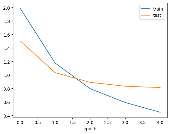
このように誤差(loss)が徐々に下がっていれば成功です。
まだ少し学習回数(epoch)を増やしても良さそうですね。
予測結果
model.eval()
preds = []
labels = []
with torch.no_grad():
    for batch in tqdm(test_loader):
        image = batch[0].to(DEVICE)
        label = batch[1].to(DEVICE)
        # 最も値の大きい列番号
        preds += model(image).cpu().numpy().argmax(axis = 1).tolist()
        # 答え
        labels += label.cpu().numpy().tolist()
modelに画像データを入れたら予測を出力します。
ただし、出力は(データ数, ラベル数)になっています。
最も値が大きい列番号が予測ラベルになるので、argmaxで取り出しましょう。
予測結果は以下のとおりです。
plt.figure(figsize = (12, 4))
for i in range(5):
    plt.subplot(1, 5, i + 1)
    plt.imshow(test[i][0].permute(1, 2, 0))
    title = f"true: {labels[i]}, pred: {preds[i]}"
    plt.title(title)
plt.tight_layout()
plt.show()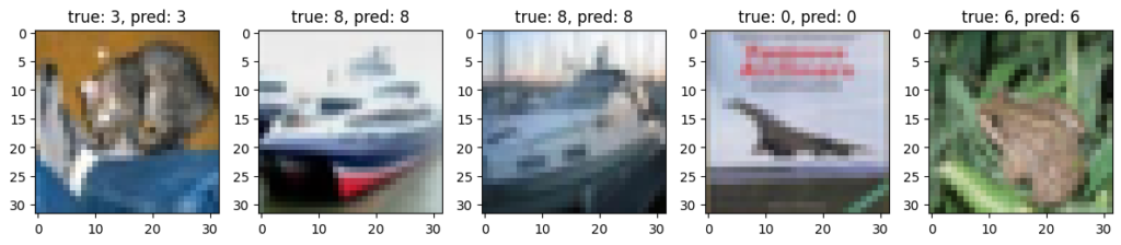
いい感じに正解していますね。
正解率も計算してみましょう。
from sklearn.metrics import accuracy_score
print(accuracy_score(labels, preds))

# ========== output ==========
# 0.7434
正解率は74%でした。
とりあえずモデルを作るだけならこれで終わりです!
残りは精度を高めるちょっとした工夫なので、興味ある方だけ読んでください。
Data Augmentation
画像モデルの学習ではData Augmentationが有効です。
何かと言うと、画像を反転させたり色を変えたりして加工しましょうということです。
image = train[0][0]
plt.subplot(1, 2, 1)
plt.imshow(image.permute(1, 2, 0))
plt.subplot(1, 2, 2)
plt.imshow(torchvision.transforms.RandomHorizontalFlip(p = 1)(image).permute(1, 2, 0))
plt.show()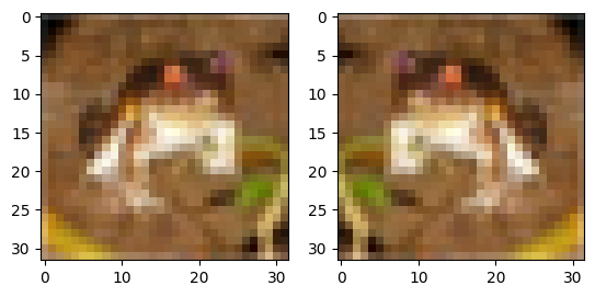
例えばtorchvisionにあるRandomHorizontalFlipを使うと、水平方向に反転してくれます。
この画像は左右どちらを向いていてもカエルであることは変わりません。
反転は学習データ(train)でのみ行えばOKです。
model = timm.create_model("resnet18d", pretrained = True, num_classes = 10).to(DEVICE)

#from tqdm import tqdm

# 最適化手法
optimizer = torch.optim.Adam(model.parameters(), lr = 1e-4)

# 損失関数
criterion = torch.nn.CrossEntropyLoss()

# ログ記録用の変数
history = {"train": [], "test": []}

# 学習回数
for epoch in range(5):
    print("\nEpoch:", epoch)

    # 学習
    model.train()
    train_loss = 0
    for batch in tqdm(train_loader):
        optimizer.zero_grad()
        image = batch[0].to(DEVICE) #(batch_size, channel, size, size)
        label = batch[1].to(DEVICE) #(batch_size)

        image = torchvision.transforms.RandomHorizontalFlip()(image)

        preds = model(image) #(batch_size, num_class)
        loss = criterion(preds, label)
        loss.backward()
        optimizer.step()
        train_loss += loss.item()

    # 検証
    model.eval()
    test_loss = 0
    with torch.no_grad():
        for batch in tqdm(test_loader):
            image = batch[0].to(DEVICE) #(batch_size, channel, size, size)
            label = batch[1].to(DEVICE) #(batch_size)
            preds = model(image) #(batch_size, num_class)
            loss = criterion(preds, label)
            test_loss += loss.item()

    # 誤差出力
    train_loss /= len(train_loader)
    test_loss /= len(test_loader)
    print(train_loss)
    print(test_loss)
    history["train"].append(train_loss)
    history["test"].append(test_loss)

plt.plot(history["train"], label = "train")
plt.plot(history["test"], label = "test")
plt.xlabel("epoch")
plt.legend()
plt.show()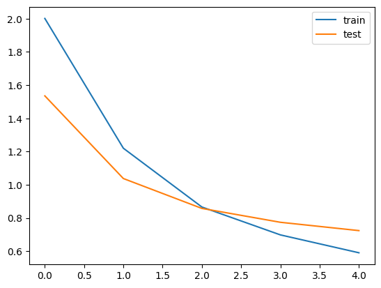
反転なしの場合よりもちょっと精度が良くなっていそうですね。
model.eval()
preds = []
labels = []
with torch.no_grad():
    for batch in tqdm(test_loader):
        image = batch[0].to(DEVICE)
        label = batch[1].to(DEVICE)
        # 最も値の大きい列番号
        preds += model(image).cpu().numpy().argmax(axis = 1).tolist()
        # 答え
        labels += label.cpu().numpy().tolist()

#from sklearn.metrics import accuracy_score
print(accuracy_score(labels, preds))

# ========== output ==========
# 0.7525
このように正解率も上がっているはずです。
他にも上下反転や回転、色の変更など様々な変換があるので、気になったら試してください。
まとめ
今回はpytorchとtimmを使って画像分類をする方法について解説しました。
これぞAIっぽい内容なので、勉強のモチベが上がりますね。


コメント