
BERTは文章を使ったタスクで主流のモデルです。
BERTの計算は非常に重いので、通常のノートPCに入っているようなCPUの計算だけではほとんど実装できません。
Google Colaboratoryを使えばGPUで計算ができます。
>>Google Colaboratoryの使い方
今回紹介するコードをコピペするだけで実装できるので、初心者でも大丈夫です。
データセット
そもそも都合よく文章データを持っていることも少ないので、
scikit-learnに入っているデータを使いましょう。
from sklearn.datasets import fetch_20newsgroups
import pandas as pd

train_data = fetch_20newsgroups(subset = 'train')
test_data = fetch_20newsgroups(subset = 'test')

train = pd.DataFrame({"text" : train_data["data"], "target" : train_data["target"]})
test = pd.DataFrame({"text" : test_data["data"], "target" : test_data["target"]})

train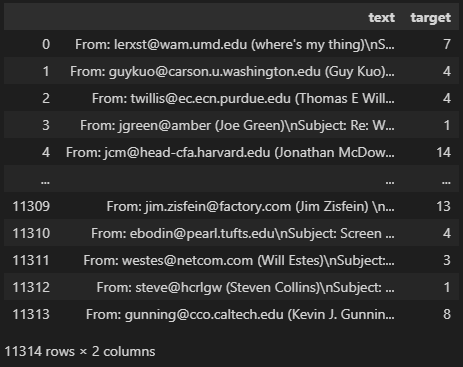
”fetch_20newsgroups”は文章分類のためのデータです。
各文章に0~19の数値ラベルがついており、文章のジャンルごとにわけられています。
たとえば1つ目の文章は以下のとおり。
print(train["text"].values[0])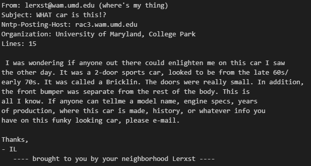
メールみたいですね。ラベルは”target”に入っており7です。
print(sorted(train["target"].unique()))
print(sorted(test["target"].unique()))

# ========== output ==========
# [0, 1, 2, 3, 4, 5, 6, 7, 8, 9, 10, 11, 12, 13, 14, 15, 16, 17, 18, 19]
# [0, 1, 2, 3, 4, 5, 6, 7, 8, 9, 10, 11, 12, 13, 14, 15, 16, 17, 18, 19]
“target”は0 ~ 19までの数値になっています。
つまり、文章から該当するラベルの数値を予測できれば成功です。
Tokenizer
機械学習では文字をデータとして入れることができず、数値にする必要があります。
BERTではtokenizerというシステムを使って、文字→数値ベクトルに変換します。
Tokenizer作成
!pip install transformers
from transformers import AutoTokenizer

MODEL_NAME = "microsoft/deberta-base"
tokenizer = AutoTokenizer.from_pretrained(MODEL_NAME)
BERTには色々なモデルがあって、今回使うdebertaはその1つです。
AutoTokenizerにモデル名を入れるとtokenizerを作成できます。
実際に変換を試してみましょう。
text = train["text"].values[0]

encoded = tokenizer(text)
print(encoded.keys())

# ========== output ==========
# dict_keys(['input_ids', 'token_type_ids', 'attention_mask'])input_ids
input_ids = encoded["input_ids"]
print(len(input_ids))
print(input_ids[:10])

# ========== output ==========
# 213
# [1, 7605, 35, 784, 254, 1178, 620, 1039, 605, 424]
input_idsは、単語をトークンと呼ばれるidに変換したものです。
単語数が多いほどidの数も増えます。
print(tokenizer.decode([7605]))

# ========== output ==========
# From
このように、例えば”From”という単語は7605に変換されています。
print(tokenizer.decode(input_ids))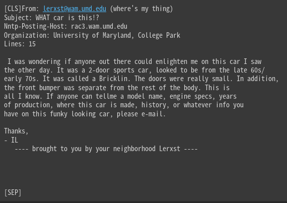
[CLS]と[SEP]が追加されています。
このようにtokenizerを通して文字を数値に変換することができます。
attention_mask
attention_mask = encoded["attention_mask"]
print(len(attention_mask))
print(attention_mask[:10])
print(attention_mask[-10:])

# ========== output ==========
# 213
# [1, 1, 1, 1, 1, 1, 1, 1, 1, 1]
# [1, 1, 1, 1, 1, 1, 1, 1, 1, 1]
attention_maskは、学習時に使用するトークンと無視するトークンを識別するものです。
1なら使用し、0なら無視されます。
今はすべて1で、その数はinput_idsと同じです。
例えば、後で解説するパディングで追加されたダミーのidは学習に不要なので、
attention_mask = 0になります。
token_type_ids
token_type_ids = encoded["token_type_ids"]
print(len(token_type_ids))
print(token_type_ids[:10])
print(token_type_ids[-10:])

# ========== output ==========
# 213
# [0, 0, 0, 0, 0, 0, 0, 0, 0, 0]
# [0, 0, 0, 0, 0, 0, 0, 0, 0, 0]
token_type_idsは、文章を2つ入力するときに使用します。
1つ目の文章にあるトークンは0、2つ目の文章にあれば1になります。
2つの文章をインプットしたい場合に活用されますが、今回は1つだけなので意味がありません。
例えば2つの文章を入れて、
その2つが同じカテゴリのものか二値分類するモデルを作るときに使用されます。
パディング
ベクトル化されたidの数は、元の文章の長さに依存します。
以下の1つ目の文章と2つ目の文章とではidの数が異なります。
text1 = train["text"].values[0]
text2 = train["text"].values[1]

encoded = tokenizer(text1)
print(len(encoded["input_ids"]))

encoded = tokenizer(text2)
print(len(encoded["input_ids"]))

# ========== output ==========
# 213
# 240
しかし、機械学習モデルを作る際は、全データの次元(列数)を統一する必要があります。
ここでいったん全文章を変換した場合の長さを見てみましょう。
import numpy as np
import matplotlib.pyplot as plt

lens = []
for text in train["text"].values:
    encoded = tokenizer.encode_plus(text.lower())
    lens.append(len(encoded["input_ids"]))
plt.hist(lens)
plt.show()

lens = np.array(lens)
print(np.percentile(lens, 50))
print(np.percentile(lens, 75))

# ========== output ==========
# 377
# 583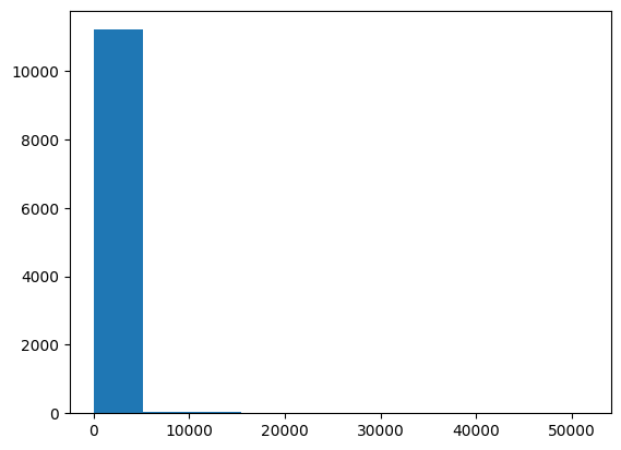
10,000を超える長さの文章もありますね。
すべての文章を最大の長さに統一してもいいですが、そうすると計算が遅くなるので、
今回は最長で512にしておきましょう。
75%の長さで583なので、512あればおおよその文章がカバーできるはずです。
MAX_LEN = 512

text = train["text"].values[0]
encoded = tokenizer(text, padding = "max_length", max_length = MAX_LEN, truncation = True)
print(len(encoded["input_ids"]))
print(encoded["input_ids"][-10:])
print(encoded["attention_mask"][:10])
print(encoded["attention_mask"][-10:])

print(tokenizer.decode(encoded["input_ids"]))

# ========== output ==========
# 512
# [0, 0, 0, 0, 0, 0, 0, 0, 0, 0]
# [1, 1, 1, 1, 1, 1, 1, 1, 1, 1]
# [0, 0, 0, 0, 0, 0, 0, 0, 0, 0]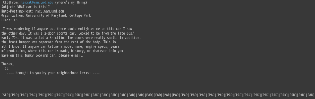
[SEP]の後を見てみると、[PAD]が追加されています。
要するに、MAX_LEN=512の長さになるまで[PAD]で埋めているわけです。
そして[PAD]の”attention_mask”は0になるので、AIモデルは無視してくれます。
Dataset, DataLoader
tokenizerの仕様を理解したところで、ここから実際にデータセットの定義をしましょう。
データセットの作り方やpytorchの使い方は以下の記事で解説しています。
>>pytorchで機械学習モデルを作る方法
import torch
from torch.utils.data import Dataset, DataLoader

class CustomData(Dataset):
    def __init__(self, data, tokenizer):
        self.data = data
        self.tokenizer = tokenizer

    def __len__(self):
        return len(self.data)

    def __getitem__(self, idx):
        text = self.data["text"].values[idx]
        encoded = self.tokenizer(
            text, padding = "max_length", max_length = MAX_LEN, truncation = True)
        input_ids = torch.tensor(
            encoded["input_ids"], dtype = torch.long)
        attention_mask = torch.tensor(
            encoded["attention_mask"], dtype = torch.long)

        label = self.data["target"].values[idx]
        label =  torch.tensor(label, dtype = torch.long)
        return {
            "input_ids": input_ids,
            "attention_mask": attention_mask,
            "label": label,
        }
これでデータセットを定義しました。
今回使う文章は1つずつなのでtoken_type_idsは不要です。
実際に出力を見てみましょう。
train_data = CustomData(train, tokenizer)
test_data = CustomData(test, tokenizer)

sample = train_data[0]
for k, v in sample.items():
    print(k, v.shape)

# ========== output ==========
# input_ids torch.Size([512])
# attention_mask torch.Size([512])
# label torch.Size([])
0を入れるとidx=0として__getitem__が実行されます。
出力サイズはMAX_LENでパディングされているので、今は512です。
train_dl = DataLoader(train_data, batch_size = 8, shuffle = True, drop_last = True)
test_dl = DataLoader(test_data, batch_size = 16, shuffle = False, drop_last = False)

batch = next(iter(train_dl))
for k, v in batch.items():
    print(k, v.shape)

# ========== output ==========
# input_ids torch.Size([8, 512])
# attention_mask torch.Size([8, 512])
# label torch.Size([8])
一気に全部のデータを読み込むとメモリがパンクするので、DataLoaderで小出しします。
1バッチを取り出してサイズを見ると、([バッチサイズ, MAX_LEN])になっています。
モデル作成
モデルの定義をします。
AutoModelにtokenizerのときと同じモデル名を入れましょう。
from torch import nn
from transformers import AutoModel

class CustomModel(nn.Module):
    def __init__(self):
        super().__init__()
        self.bert = AutoModel.from_pretrained(MODEL_NAME)
        self.head = nn.Linear(in_features = 768, out_features = 20) # クラス数

    def forward(self, input_ids, attention_mask):
        outputs = self.bert(
            input_ids = input_ids,
            attention_mask = attention_mask,
        ) # [batch_size, max_len, 768]
        x = outputs.last_hidden_state[:, 0, :] # cls_token
        logits = self.head(x)
        return logits
BERTの出力はちょっと複雑で説明しきれないので、検索してみると良いです。
last_hidden_stateという出力が使いやすいです。
その出力サイズは[batch_size, max_len, 768]で、max_lenの先頭[0]はcls_tokenと呼ばれます。
cls_tokenは文章全体の特徴を持っています。
なので使用する出力サイズは[batch_size, 768]で、そこからLinearでラベル数20にしました。
学習
pytorchの学習方法についても以下の記事を参考にしてください。
>>pytorchで機械学習モデルを作る方法
まず、計算が重いのでGPUを設定します。
GPUを持っていない人はGoogle Colaboratoryを使えばOKです。
ここでGPU(T4)にしましょう。
DEVICE = "cuda" if torch.cuda.is_available() else "cpu"
print(DEVICE)
DEVICE=”cuda”になっていればGPUが使えています。
仮に使えてなくてもコードは動きますが、計算が重すぎて終わらないかもしれません。
以下のコードで学習を実行します。
DEVICE = "cuda" if torch.cuda.is_available() else "cpu"
print(DEVICE)

import matplotlib.pyplot as plt
from tqdm import tqdm

# モデル呼び出し
model = CustomModel().to(DEVICE)

# 最適化手法
optimizer = torch.optim.Adam(model.parameters(), lr = 2e-6)

# 損失関数
criterion = nn.CrossEntropyLoss()

# 学習ログを保存する変数
history = {"train": [], "test": []}

# epochの数だけ学習を繰り返す
for epoch in range(5):

    # 学習
    model.train()
    train_loss = 0
    for batch in tqdm(train_dl):
        optimizer.zero_grad()
        input_ids = batch["input_ids"].to(DEVICE)
        attention_mask = batch["attention_mask"].to(DEVICE)
        label = batch["label"].to(DEVICE)
        logits = model(input_ids, attention_mask)
        loss = criterion(logits, label) # 誤差計算
        loss.backward()                 # 誤差伝播
        optimizer.step()                # パラメータ更新
        train_loss += loss.item()
    train_loss /= len(train_dl)

    # 検証
    model.eval()
    test_loss = 0
    with torch.no_grad(): # パラメータ更新をしない
        for batch in tqdm(test_dl):
            input_ids = batch["input_ids"].to(DEVICE)
            attention_mask = batch["attention_mask"].to(DEVICE)
            label = batch["label"].to(DEVICE)
            logits = model(input_ids, attention_mask)
            loss = criterion(logits, label)
            test_loss += loss.item()
    test_loss /= len(test_dl)

    # ログ保存
    history["train"].append(train_loss)
    history["test"].append(test_loss)

    print("TrainLoss:", train_loss)
    print("TestLoss:", test_loss)

plt.plot(history["train"], label = "train")
plt.plot(history["test"], label = "test")
plt.legend()
plt.show()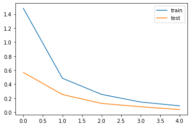
ちょっとずつlossが下がっていれば成功です。
学習率(lr)をかなり小さめの2e-6にしています。大きいとうまく学習してくれません。
予測
preds = []
model.eval()
with torch.no_grad():
    for batch in tqdm(test_dl):
        input_ids = batch["input_ids"].to(DEVICE)
        attention_mask = batch["attention_mask"].to(DEVICE)
        logits = model(input_ids, attention_mask)
        preds.append(nn.Softmax(dim = 1)(logits).cpu().numpy())
preds = np.concatenate(preds, axis = 0)
予測は検証時と同じことをして、モデルの出力を取り出しておけばOKです。
Softmaxを列方向にかけて、各ラベルに該当する確率にしましょう。
print(preds[0])
print(test["target"].values[0])

# ========== output ==========
# [1.14693976e-04 3.06718430e-04 1.77172536e-04 5.27597358e-03
#  1.53868657e-03 5.80334636e-05 3.96165112e-03 9.84234631e-01
#  1.41639716e-03 6.91743699e-05 7.64065262e-05 4.37081435e-05
#  1.64264045e-03 2.19690846e-04 9.28332156e-05 9.14977572e-05
#  1.26073413e-04 9.59314420e-05 3.28952592e-04 1.29076332e-04]
# 7
このように20ラベルそれぞれの確立になっています。
よく見たら8番目(0, 1, 2, …と数える)の確率が0.98で高いですね。
pred_labels = preds.argmax(axis = 1)

print(pred_labels[:5])
print(test["target"].values[:5])

# ========== output ==========
# [ 7  5  0 17 19]
# [ 7  5  0 17 19]
argmaxを列方向に適用し、最も確立の大きい列番号を予測ラベルとしました。
あっていそうですね。
正解率を計算してみましょう。
from sklearn.metrics import accuracy_score

print(accuracy_score(test["target"].values, pred_labels))

# ========== output ==========
# 0.846255974508762784.6%ですね。ちなみにLightGBMで作ったモデルの精度は高くて66%でした。
BERTのほうが精度が高いモデルを作りやすいですが、計算が重いことが難点ですね。
まとめ
今回はBERTの使い方を解説しました。
精度よりも計算の軽さを優先したいなら、LightGBMとtf-idfを使う方法をおすすめします。


コメント