

今回はTensorFlowでBERTモデルを作り文章分類をする方法を解説します。
“input_ids”, “attention_mask”の意味がわかれば簡単です。
データ準備
fetch_20newsgroups
from sklearn.datasets import fetch_20newsgroups
import pandas as pd

train_data = fetch_20newsgroups(subset = 'train')
test_data = fetch_20newsgroups(subset = 'test')

train = pd.DataFrame({"text" : train_data["data"], "target" : train_data["target"]})
test = pd.DataFrame({"text" : test_data["data"], "target" : test_data["target"]})

train.head()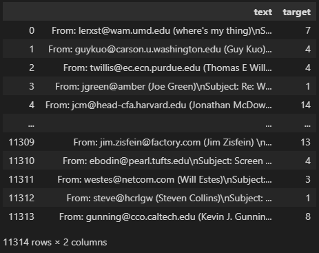
データは”fetch_20newsgroups”を使います。
文章から”target”のラベルを予測するモデルを作りましょう。
text cleaning
import re
def cleaning(text):
    text = re.sub("\n", " ", text)           # 改行削除
    text = re.sub("[^A-Za-z0-9]", " ", text) # 記号削除
    text = re.sub("[' ']+", " ", text)       # スペース統一
    return text.lower()                      # 小文字で出力

train["text_cleaned"] = train["text"].map(cleaning)
test["text_cleaned"] = test["text"].map(cleaning)

train.head()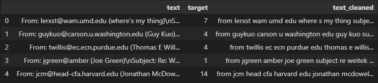
文章には改行やスペースなどが入っているので、単純になるように加工しました。
また、これから使用する”bert-base-uncased”は小文字にのみ対応しています。
なので、文章はすべて小文字に変換しておきましょう。
モデルの種類によっては大文字でも大丈夫だったりします。
Tokenizer
tokenizer
!pip install transformers
from transformers import AutoTokenizer

MODEL_NAME = "bert-base-uncased"
tokenizer = AutoTokenizer.from_pretrained(MODEL_NAME)
機械学習モデルには文章を入れることができません。
なので、文章を数値に変換する必要があります。
ここで使えるのが”tokenizer”です。
“bert-base-uncased”とう形式のtokenizerを呼び出しましょう。
これで文章を数値(ベクトル)に変換することができます。
MAX_LEN = 256

train_tokens = tokenizer.batch_encode_plus(
    train["text_cleaned"].to_list(),
    padding = "max_length",
    max_length = MAX_LEN,
    truncation = True
)

test_tokens = tokenizer.batch_encode_plus(
    test["text_cleaned"].to_list(),
    padding = "max_length",
    max_length = MAX_LEN,
    truncation = True
)

print(train_tokens["input_ids"][0][:5])
print(train_tokens["attention_mask"][0][:5])
print(train_tokens["token_type_ids"][0][:5])

# ========== output ==========
# [101, 2013, 3393, 2099, 2595]
# [1, 1, 1, 1, 1]
# [0, 0, 0, 0, 0]このように文章を”input_ids”として数値ベクトルに変換できます。
全データでベクトルの次元(列数)を統一する必要があるので、
今回は”max_length = 256″にしました。
長さが足りない文章にはパディングが追加され、超えている文章は256以降を切り捨てています。
print(tokenizer.decode(train_tokens["input_ids"][0]))
print(train_tokens["attention_mask"][0][-10:])

# ========== output ==========
# [0, 0, 0, 0, 0, 0, 0, 0, 0, 0]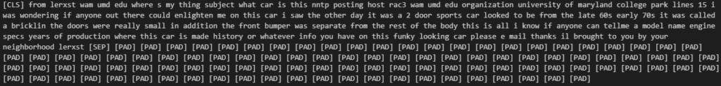
このように[PAD]が足されています。
パディングした部分は学習に使いませんので、”attention_mask = 0″となっています。
データセット
import tensorflow as tf

train_dataset = tf.data.Dataset.from_tensor_slices((
    {"input_ids": train_tokens["input_ids"],
     "attention_mask": train_tokens["attention_mask"],
     "token_type_ids": train_tokens["token_type_ids"]},
    train["target"].values
))

test_dataset = tf.data.Dataset.from_tensor_slices((
    {"input_ids": test_tokens["input_ids"],
     "attention_mask": test_tokens["attention_mask"],
     "token_type_ids": test_tokens["token_type_ids"]},
    test["target"].values
))

train_dataset = train_dataset.batch(16)
test_dataset = test_dataset.batch(16)

train_dataset = train_dataset.shuffle(1024 * 16)

batch = next(iter(train_dataset))
print(batch[0]["input_ids"].shape)
print(batch[0]["attention_mask"].shape)
print(batch[0]["token_type_ids"].shape)
print(batch[1].shape)

# ========== output ==========
# (16, 256)
# (16, 256)
# (16, 256)
# (16,)
“from_tensor_slices”にデータを渡してデータセットを作りましょう。
特徴量として”input_ids”, “attention_mask”, “token_type_ids”を辞書型で入れます。
答えは”target”をそのまま入れればOKです。
“batch”で指定した量ごとにデータを小出しするようにしています。今回は16ずつです。
“shuffle”ではデータをシャッフルしています。()の数値はデータの量以上にしておけば無難です。
バッチの中身は(データ数, max_length)になっています。
モデル作成
import tensorflow.keras.layers as L
import tensorflow.keras.models as M
from transformers import TFAutoModel

def get_model(max_length, num_classes):
    # input_idsを受け取る層
    input_ids = L.Input(
        shape = (max_length), dtype = tf.int32, name = "input_ids"
    )

    # attention_maskを受け取る層
    attention_mask = L.Input(
        shape = (max_length), dtype = tf.int32, name = "attention_mask"
    )

    # token_type_idsを受け取る層
    token_type_ids = L.Input(
        shape = (max_length), dtype = tf.int32, name = "token_type_ids"
    )

    # BERTモデル
    bert_model = TFAutoModel.from_pretrained(MODEL_NAME)
    transformer_outputs = bert_model(
        {"input_ids": input_ids,
         "attention_mask": attention_mask,
         "token_type_ids": token_type_ids}
    )
    pooler_output = transformer_outputs.pooler_output

    # BERTの出力->クラス数に変換する層
    outputs = L.Dense(units = num_classes, activation = "softmax")(pooler_output)

    # 定義した層からモデルを作成
    model = M.Model(
        inputs = [input_ids, attention_mask, token_type_ids],
        outputs = outputs
    )

    # 最適化手法と損失関数を定義
    model.compile(
        optimizer = tf.keras.optimizers.Adam(learning_rate = 1e-5),
        loss = "sparse_categorical_crossentropy"
    )
    return model

# モデルを呼び出す
tf.keras.backend.clear_session()
model = get_model(MAX_LEN, 20)
model.summary()
細かい定義の方法についてはこちらの記事で解説しています。
まず、”input_ids”, “attention_mask”, “token_type_ids”を受け取る層を定義します。
BERTの層はtransformersのTFAutoModelから呼び出すことができます。
モデルの種類はtokenizerと同じ”bert-base-uncased”にしましょう。
最初に受け取ったidたちをBERTの層に入れると、様々な出力が得られます。
今回は”pooler_output”にしました。これは768次元ある出力です。
詳しくは”BERT outputs”で検索すると色々出てきます。
最後の出力はクラス数の20にして、softmaxで確立にしておきましょう。
学習と検証
import matplotlib.pyplot as plt

checkpoint = tf.keras.callbacks.ModelCheckpoint(
    "best_weight.h5",
    monitor = "val_loss",
    direction = "min",
    save_best_only = True,
    save_weights_only = True
)

history = model.fit(
    train_dataset,
    validation_data = test_dataset,
    epochs = 5,
    callbacks = [checkpoint]
)

plt.plot(history.history["loss"], label = "train")
plt.plot(history.history["val_loss"], label = "valid")
plt.legend()
plt.show()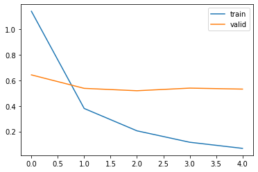
学習には時間がかかるのでGPUを使用することをおすすめします。
GPUはGoogle Colaboratoryを使うか、PCを自作して用意しましょう。
>>Google Colaboratoryの使い方
>>機械学習用自作PCの構築方法
青線の学習データは徐々にlossが下がっていますが、検証データのlossは若干増減していますね。
なので、検証データで最小のlossのときのみモデルを保存するようにしています。
予測
preds = model.predict(test_dataset)
print(preds[0])
print(test["target"].values[0])

# ========== output ==========
# [4.1645556e-04 1.4995325e-04 1.8941988e-04 1.9290292e-03 2.9584046e-02
#  1.1660752e-04 4.5209704e-04 9.6284521e-01 1.4236132e-03 3.2213202e-04
#  3.5594727e-04 1.0729847e-04 5.9568835e-04 3.1473258e-04 6.3134205e-05
#  4.0978874e-04 4.2964806e-04 1.2677899e-04 6.2931198e-05 1.0546876e-04]
# 7
“predict”で予測できます。
予測結果はラベル数と同じ次元があり、今回は20列ですね。
それぞれが各ラベルに該当する確率となっています。
pred_labels = preds.argmax(axis = 1)
print(pred_labels[:5])
print(test["target"].values[:5])

# ========== output ==========
# [ 7  5  0 17 19]
# [ 7  5  0 17 19]
“argmax”で、各行において最も値が大きい列番号を取り出しましょう。
答えと照らし合わせてみるとだいたいあっていそうですね。
from sklearn.metrics import accuracy_score
print(accuracy_score(test["target"].values, pred_labels))

# ========== output ==========
# 0.86311736590547
正解率を計算すると86.3%でした。
ちなみにCPUで計算できるLightGBMのモデルでは正解率は66.3%でした。
まとめ
今回はTensorFlowでBERTを実装する方法を解説しました。
TensorFlowはTPUが使えるので計算が重いBERTもサクサク回せるので便利です。
Pytorchでも同じモデルを作ることができます。こちらのほうがメジャーです。

コメント